BrainWave is a module containing functions to process electroencephalographic (EEG) recordings with the Julia programming language. The software is in alpha status, it is here in the hope that it may be useful to someone looking into analysing EEG data with Julia. However, currently the software unsupported, and radical API changes may occurr at any time.

BrainWave.jl Tutorial

For this tutorial, we'll use the example dataset contained in the EEGLab distribution. You can download a copy of EEGLab from here. After unzipping the file, copy the "eeglab_data.set", and "eeglab_chan32.locs" files from the "sample_data" directory to the directory you want to work with julia. The first file contains the EEG data, while the second file contains information about the channel locations.

After starting julia we load the modules that we need. We'll use the MAT.jl module to read in the EEGLab dataset that is saved in the MATLAB MAT format.

using BrainWave, MAT, PyPlot

We'll start by reading in the channel labels, which are stored in the fourth column of a simple tab-delimited text file:

chanTab = readdlm("eeglab_chan32.locs", '\t')
chanLabels = chanTab[:,4]

we'll also strip the chanLabels strings from any leading/trailing whitespace with the following command:

[chanLabels[i] = strip(chanLabels[i]) for i=1:length(chanLabels)]

the fourth and sixth labels are empty, if you look at the "eeglab_chan32.locs" file (with a text editor or a spreadsheet application) you'll see that the labels for these channels, which are the EOG channels, are stored in the fifth column of the file. We'll add them to our chanLabels with the following commands:

chanLabels[2] = "EOG1"; chanLabels[6] = "EOG2"

Now we read in the EEGLab dataset:

fileIn = matopen("eeglab_data.set")
dset = read(fileIn, "EEG")
close(fileIn)

If you inspect the dset variable you'll see that it is a dictionary with 30 entries. The most important fields are the dset["data"] field which contains the data, and the dset["event"] field, which contains information about the experimental events. The dset["event"] field contains two subfields, the dset["event"]["type"] field, which contains the trigger codes, and the dset["event"]["latency"] field, which contains the timing of the trigger codes (measured not in seconds or milliseconds, but in terms of number of samples from the start of the recording). The triggers in this dataset are coded as strings, the experimental events that are stored in dset["event"]["type"] are either "square", or "rt". I won't go in to the details of what these represent, you can read the EEGLab tutorial if you're interested. Currently BrainWave doesn't support triggers coded as strings, so we'll convert them to numbers, 1 for "square", and 2 for "rt". We'll organize the information about the experimental events in an event table, which is a dictionary with fields code, for the trigger codes, and idx for the sample numbers:

nEvents = length(dset["event"]["type"]) #count how many events we have
code = zeros(Int, nEvents) #prepare array to store trigger codes
idx = zeros(Int, nEvents) #prepare array to store sample numbers
for i=1:nEvents
    idx[i] = round(Int, dset["event"]["latency"][i])
    code[i] = ifelse(dset["event"]["type"][i] == "square", 1, 2)
end

#create event table
evtTab = Dict{String,Any}("code" => code,
                          "idx" => idx)

next we store the data in a variable called data, and the sampling rate of the recording in a variable called sampRate:

data = dset["data"]
sampRate = round(Int, dset["srate"])

if you inspect the data variable, you'll see that it is simply a 2-dimensional array of floating point numbers, where each row represents a channel, and each column is a sample point. In our case, we have 32 channels, and 3054 sample points, which at a sampling rate of 128-Hz correspond to about 238 seconds of recording:

size(data, 2) / sampRate

238.3125

We'll re-reference the data to an average reference, but excluding the EOG1 and EOG2 channels

idxEOG = [find(chanLabels .== "EOG1")[1], find(chanLabels .== "EOG2")[1]]
data = data .- mean(deleteSlice2D(data, idxEOG, 1), 1)

Next, we'll filter the recording with a bandpass filter between 1 and 30 Hz:

filterContinuous!(data, sampRate, "bandpass", 512, [1, 30], transitionWidth=0.2)

We'll then epoch the recording:

epochStart = -1
epochEnd = 2
segs, nRaw = segment(data, evtTab, epochStart, epochEnd,
                     sampRate, eventsList=[1])

and baseline correct:

baselineCorrect!(segs, epochStart, abs(epochStart), sampRate)

We move on to detect artefacts and remove them:

thresh = 75
toRemoveDict = findArtefactThresh(segs, thresh)
removeEpochs!(segs, toRemoveDict)

Next we average the epochs to obtain the ERP:

ave, nSegs = averageEpochs(segs)

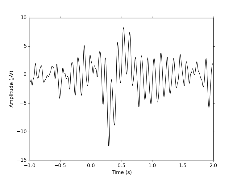
and plot the ERP:

tArr = collect(0:size(ave["1"],2)-1)/sampRate + epochStart
plot(tArr, ave["1"][find(chanLabels .== "POz")[1],:], color="black")
xlabel("Time (s)"); ylabel(L"Amplitude ($\mu$V)")