This page describes some basic sound processing functions in R. We’ll use the tuneR package to read in wav files. No other packages will be needed for this tutorial, however, there is a number of packages that are in general very useful for working with sound in R:

• signal – MATLAB like signal processing functions
• seewave – functions for analysing, manipulating, displaying, editing and synthesizing time waves (particularly sound).

We can install the sound package with

install.packages('tuneR', dep=TRUE)

Assuming that the tuneR package has already been installed correctly we can load it with the library() function

library(tuneR)

Now we can read in a wav file, you can download it here 440_sine.wav, it contains a complex tone with a 440 Hz fundamental frequency (F0) plus noise.

sndObj <- readWave('440_sine.wav')

sndObj is an object of class Wave, we can inspect its properties with the following command:

> str(sndObj)
Formal class 'Wave' [package "tuneR"] with 5 slots
  ..@ left     : int [1:5292] 0 0 0 0 0 0 0 0 0 0 ...
  ..@ right    : int [1:5292] 0 0 0 0 0 0 0 0 0 0 ...
  ..@ stereo   : logi TRUE
  ..@ samp.rate: int 44100
  ..@ bit      : int 16

the wav file has two channels (@left and @right) containing 5060 sample points each, considering the sample rate ([email protected] = 44110) this corresponds to a duration of 120 ms:

> 5292 / [email protected]
[1] 0.12

we’ll select and work only with one of the channels from now onwards:

s1 <- sndObj@left

the readWave function reads wav files as integer types. Our wav file has a 16-bit depth (sndObj@bit), this means that the sound pressure values are mapped to integer values that can range from -2^15 to (2^15)-1. We can convert our sound array to floating point values ranging from -1 to 1 as follows:

s1 <- s1 / 2^(sndObj@bit -1)

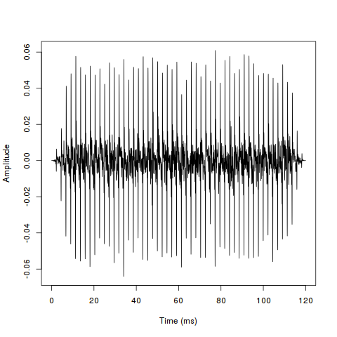
Plotting the Tone

A time representation of the sound can be obtained by plotting the pressure values against the time axis. However we need to create an array containing the time points first:

timeArray <- (0:(5292-1)) / [email protected]
timeArray <- timeArray * 1000 #scale to milliseconds

now we can plot the tone:

plot(timeArray, s1, type='l', col='black', xlab='Time (ms)', ylab='Amplitude') 

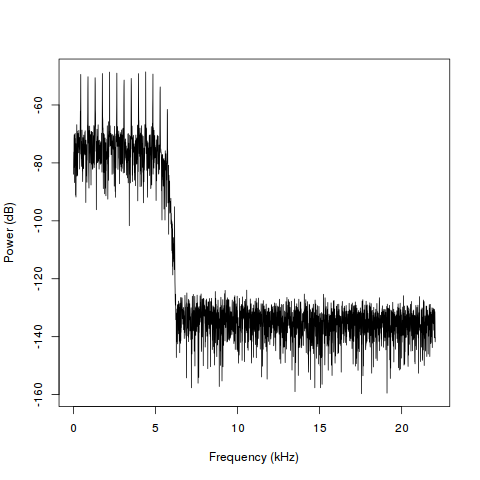
Plotting the Frequency Content

Another useful graphical representation is that of the frequency content, or spectrum of the tone. We can obtain the frequency spectrum of the sound using the fft function, that implements a Fast Fourier Transform algorithm. We’ll follow closely the technical document available here to obtain the power spectrum of our sound.

n <- length(s1)
p <- fft(s1)

the fft is computed on the number of points of the signal n. Since we’re not using a power of two the computation will be a bit slower, but for signals of this duration this is negligible.

nUniquePts <- ceiling((n+1)/2)
p <- p[1:nUniquePts] #select just the first half since the second half 
                     # is a mirror image of the first
p <- abs(p)  #take the absolute value, or the magnitude 

the fourier transform of the tone returned by the fft function contains both magnitude and phase information and is given in a complex representation (i.e. returns complex numbers). By taking the absolute value of the fourier transform we get the information about the magnitude of the frequency components.

p <- p / n #scale by the number of points so that
           # the magnitude does not depend on the length 
           # of the signal or on its sampling frequency  
p <- p^2  # square it to get the power 

# multiply by two (see technical document for details)
# odd nfft excludes Nyquist point
if (n %% 2 > 0){
  p[2:length(p)] <- p[2:length(p)]*2 # we've got odd number of points fft
} else {
  p[2: (length(p) -1)] <- p[2: (length(p) -1)]*2 # we've got even number of points fft
}

freqArray <- (0:(nUniquePts-1)) * ([email protected] / n) #  create the frequency array 

plot(freqArray/1000, 10*log10(p), type='l', col='black', xlab='Frequency (kHz)', ylab='Power (dB)')

The resulting plot can bee seen below, notice that we’re plotting the power in decibels by taking 10*log10(p), we’re also scaling the frequency array to kilohertz by dividing it by 1000

To confirm that the value we have computed is indeed the power of the signal, we’ll also compute the root mean square (rms) of the signal. Loosely speaking the rms can be seen as a measure of the amplitude of a waveform. If you just took the average amplitude of a sinusoidal signal oscillating around zero, it would be zero since the negative parts would cancel out the positive parts. To get around this problem you can square the amplitude values before averaging, and then take the square root (notice that squaring also gives more weight to the extreme amplitude values):

> rms_val <- sqrt(mean(s1^2))
> rms_val
[1] 0.01382841

since the rms is equal to the square root of the overall power of the signal, summing the power values calculated previously with the fft over all frequencies and taking the square root of this sum should give a very similar value

> sqrt(sum(p))
[1] 0.01382841

References

• Hartmann, W. M. (1997), Signals, Sound, and Sensation. New York: AIP Press
• Plack, C.J. (2005). The Sense of Hearing. New Jersey: Lawrence Erlbaum Associates.
• The MathWorks support. Technical notes 1702, available: https://web.archive.org/web/20120615002031/http://www.mathworks.com/support/tech-notes/1700/1702.html